DLS is a useful tool for anyone developing biologics or gene therapies. Complex biological samples such as enzymes, monoclonal antibodies, or AAVs that will be used for treatments must be highly stable for storage, transport, and clinical administration.
DLS enables you to monitor the colloidal stability of your sample. This information helps you optimize your sample by making changes to the sequence or buffer environment, and measuring how those changes impact colloidal stability.
PDI, or the Polydispersity Index, is a value that reflects how much variation is present in your sample. A PDI close to zero means a single, tightly-folded species that is highly regular between individual particles. As the PDI increases, it indicates that your macromolecules are imperfectly folded, aggregating, or contain contaminant particles.
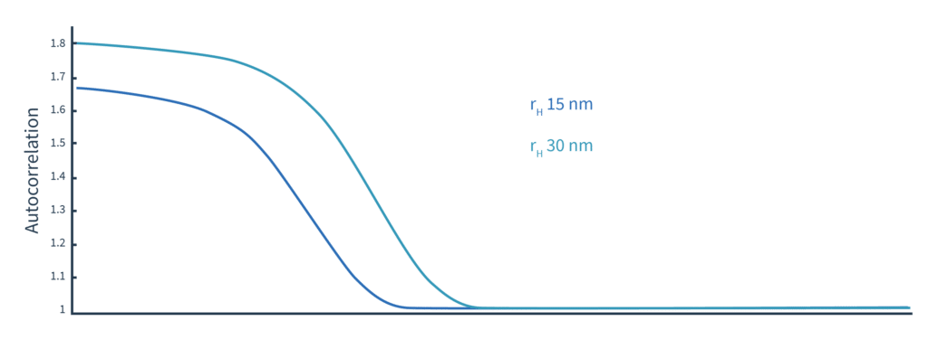
ACF and ACF fit for two different samples, containing a single population of different sized beads. The decay function changes based on the size of particles in solution.
Overlaid size distribution plots resulting from the ACF fit data calculated for each particle size. Dotted lines represent the cumulant radius of each population. Note that the cumulant radius aligns well with the size distribution peaks, representing single, tightly-folded populations.
Particles move at different speeds and scatter different amounts of light based on their size. Larger particles move slower and scatter more light compared to smaller particles. DLS optics are very sensitive, and measure the intensity fluctuations of light from a sample.
The autocorrelation function, or ACF, captures the information about the fluctuations of scattered light. The decay data is plotted, and a line is fit through the data – the ACF fit. This fit is mathematically converted into plots that convey information about the average size of particles in a solution, as well as the distribution of particle sizes in a given sample.
You will use different fit models depending on the quality of your sample. Samples containing only a single population of particles use the cumulant radius fit. Those with multiple populations present are better suited for a size distribution fit.
ACF data (black dots) with size distribution ACF fit (teal) and cumulant radius ACF fit (blue) for a sample with multiple particle sizes present.
Size distribution plot showing different sized populations within the sample (solid). Cumulant radius fit for a single population shown (dashed).
Prometheus Panta offers a combinatorial approach to protein optimization that includes DLS optics. Learn more about the instrument and how it works.